Lab 7(a): Grid Localization using Bayes Filter
Objective
The goal is to implement grid localization using Bayes Filter.
Code
# In world coordinates
def compute_control(cur_pose, prev_pose):
    """ Given the current and previous odometry poses, this function extracts
    the control information based on the odometry motion model.

    Args:
        cur_pose  ([Pose]): Current Pose
        prev_pose ([Pose]): Previous Pose

    Returns:
        [delta_rot_1]: Rotation 1  (degrees)
        [delta_trans]: Translation (meters)
        [delta_rot_2]: Rotation 2  (degrees)
    """

    xprev = prev_pose[0]; yprev = prev_pose[1]; thprev = prev_pose[2]
    xcurr = cur_pose[0]; ycurr = cur_pose[1]; thcurr = cur_pose[2]

    delta_rot_1 = np.arctan2(ycurr - xcurr,xcurr - xprev) - thprev
    delta_trans = np.sqrt((ycurr-yprev)**2 + (xcurr-xprev)**2)
    delta_rot_2 = thcurr-thprev-delta_rot_1

    return delta_rot_1, delta_trans, delta_rot_2

# In world coordinates
def odom_motion_model(cur_pose, prev_pose, u):
    """ Odometry Motion Model

    Args:
        cur_pose  ([Pose]): Current Pose
        prev_pose ([Pose]): Previous Pose
        (rot1, trans, rot2) (float, float, float): A tuple with control data in the format
                                                   format (rot1, trans, rot2) with units (degrees, meters, degrees)


    Returns:
        prob [float]: Probability p(x'|x, u)
    """
    # Odom
    [rot1_o,trans_o,rot2_o] = compute_control(cur_pose, prev_pose)

    # Given States
    rot1_s =  u[0];  trans1_s = u[1]; rot2_s = u[2]

    # Calculate error, mean and std dev
    err1 = rot1_o - rot1_s; err2 = trans_o - trans_s; err3 = rot2_o - rot2_s
    var1 = odom_rot_sigma; var2 = odom_trans_sigma; var3 = odom_rot_sigma

    # Find probability for each
    p1 = gaussian(err1,mean1,var1)
    p2 = gaussian(err2,mean2,var2)
    p3 = gaussian(err3,mean3,var3)

    # Total probability
    prob = np.multiply(p1,p2,p3)

    return prob

def prediction_step(cur_odom, prev_odom,xt):
    """ Prediction step of the Bayes Filter.
    Update the probabilities in loc.bel_bar based on loc.bel from the previous time step and the odometry motion model.

    Args:
        cur_odom  ([Pose]): Current Pose from odom
        prev_odom ([Pose]): Previous Pose from odom
        xt ([Pose]): Current State
    """
    # Control input
    u = compute_control(cur_odom, prev_odom)

    # Grid
    grid = obs_views

    # Initialize prev_pose to be 3d numpy array
    prev_pose = np.zeros(3)

    # PREVIOUS POSE
    s = 0
    # Iterate thru all possible x
    for xp in range(0,MAX_CELLS_X-1):
        # Iterate thru all possible y
        for yp in range(0,MAX_CELLS_Y-1):
            # Iterate thru all possible th
            for thp in range (0,MAX_CELLS_A-1):

                # Get prev pose ( Take mean of all observations)
                for i in range [0,17]:
                    prev_pose[xp,yp,thp] = prev_pose[xp,yp,thp] + grid[xp,yp,thp,i]
                prev_pose = prev_pose/18

                # Calculate probability
                p = odom_motion_model(xt, prev_pose, u)

                # Calculate belief
                s = s + p*loc.bel(xc,yc,thc)

    loc.bel_bar(xc,yc,thc) = s


def sensor_model(obs,xt):
    """ This is the equivalent of p(z|x).


    Args:
        obs ([ndarray]): A 1D array consisting of the measurements made in rotation loop

    Returns:
        [ndarray]: Returns a 1D array of size 18 (=loc.OBS_PER_CELL) with the likelihood of each individual measurements
        xt ([Pose]): Current State
    """

    # Get expected sensor readings at this pose
    expected = get_views(xt[0],xt[1],xt[2])

    # Iterate thru sensor measurments
    for m in range(0,OBS_PER_CELL-1)

        # Find probability given actual measurements
        prob[m] = gaussian(obs[m] - expected[m], 0 , sensor_sigma)

    return prob_array

def update_step(xt,obs):
    """ Update step of the Bayes Filter.
    Update the probabilities in loc.bel based on loc.bel_bar and the sensor model.
    xt ([Pose]): Current State
    obs ([ndarray]): A 1D array consisting of the measurements made in rotation loop
    """

    # Define eda
    eda = 1

    # Compute probability
    pz_t = sensor_model(obs,xt)

    # Compute belief
    loc.bel = eda*np.multiply(pz_t,loc.bel_bar)
Lab 7(b): Mapping
Objective
The purpose of this lab is to build up a map of a room.Map
Steps
-
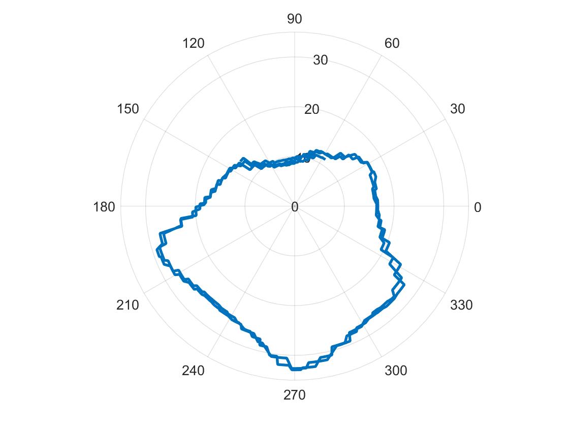
Plotted the output as a polar coordinate plot as shown below. However, I had to alter the lower velocity to something higher since the battery I switched to provided a lower power than the battery I swapped out. I didn't wait for the TOF sensor data to be ready to save time in computing. The biggest source of inconsistency is that to achieve proper readings, I lowered the velocity which added a drift away from the center of mass to be the rotation point.
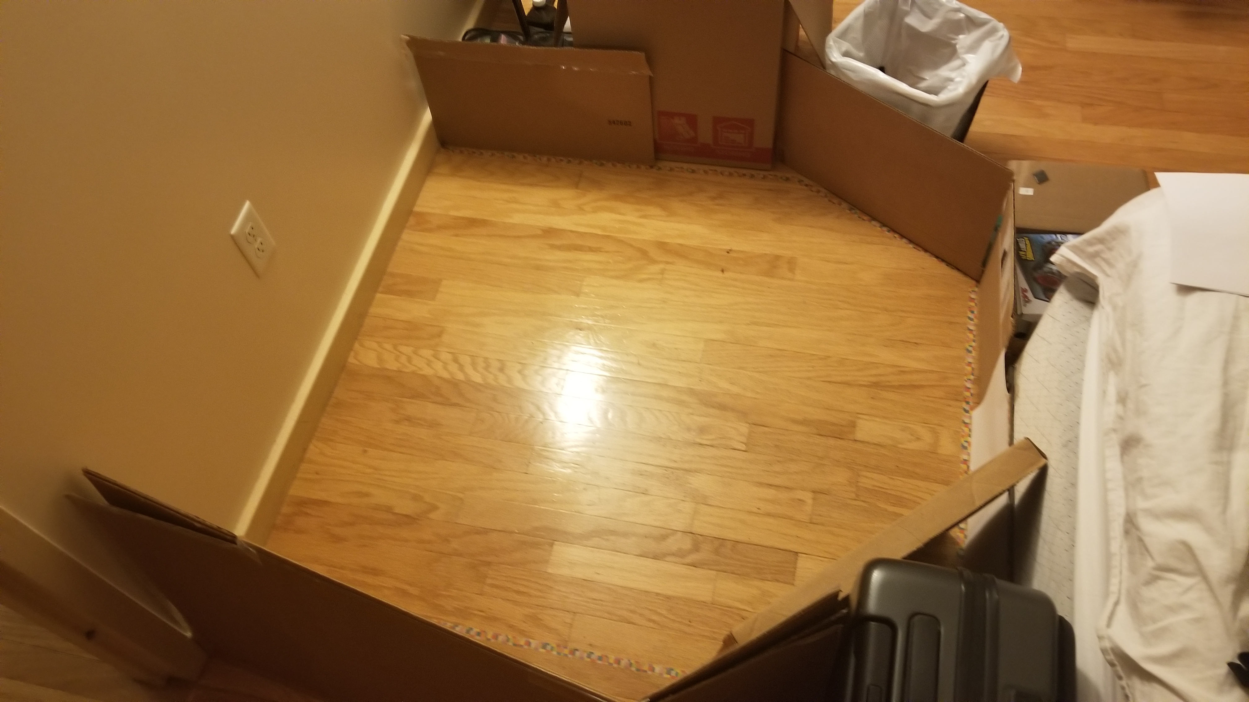
For the most part, the image shown above resembles the actual map pretty closely.
Code
if (bytestream_active) { // ------------------------ Distance sensor ------------------------ // distanceSensor.startRanging(); //Write configuration bytes to initiate measurement distance = distanceSensor.getDistance(); //Get the result of the measurement from the sensor distanceSensor.clearInterrupt(); distanceSensor.stopRanging(); float distanceMM = distance; // ------------------------ Send Data ------------------------ // res_cmd->command_type = BYTESTREAM_TX; res_cmd->length = 14; //TODO: Put an example of a 32-bit integer and a 64-bit integer //for the stream. Be sure to add a corresponding case in the //python program. timecurr = millis(); memcpy(res_cmd->data, &timecurr, 4); // time memcpy(res_cmd->data + 4, &th, 4); memcpy(res_cmd->data + 8, &distanceMM, 8); amdtpsSendData((uint8_t *)res_cmd, 14); // ------------------------ measure ang.vel ------------------------ // if ( myICM.dataReady() ) { myICM.getAGMT(); // The values are only updated when you call 'getAGMT' dt = (timecurr - timeprev) / 1000; timeprev = timecurr; th = th + (myICM.gyrZ()) * dt; // ------------------------ PID ------------------------ // myPID.Compute(); // ------------------------ Move Motors at Steady speeds ------------------------ // Rightspeed = min(150, Output + 60); Leftspeed = min(150, Output + 60); myMotorDriver.setDrive( LEFT_MOTOR, 1, Leftspeed); //Drive motor i forward at full speed myMotorDriver.setDrive( RIGHT_MOTOR, 1, Rightspeed); //Drive motor i forward at full speed } } -
Using the following transformation matrix from class (assuming the robot's starting position is the inertial frame for the data from the last part):
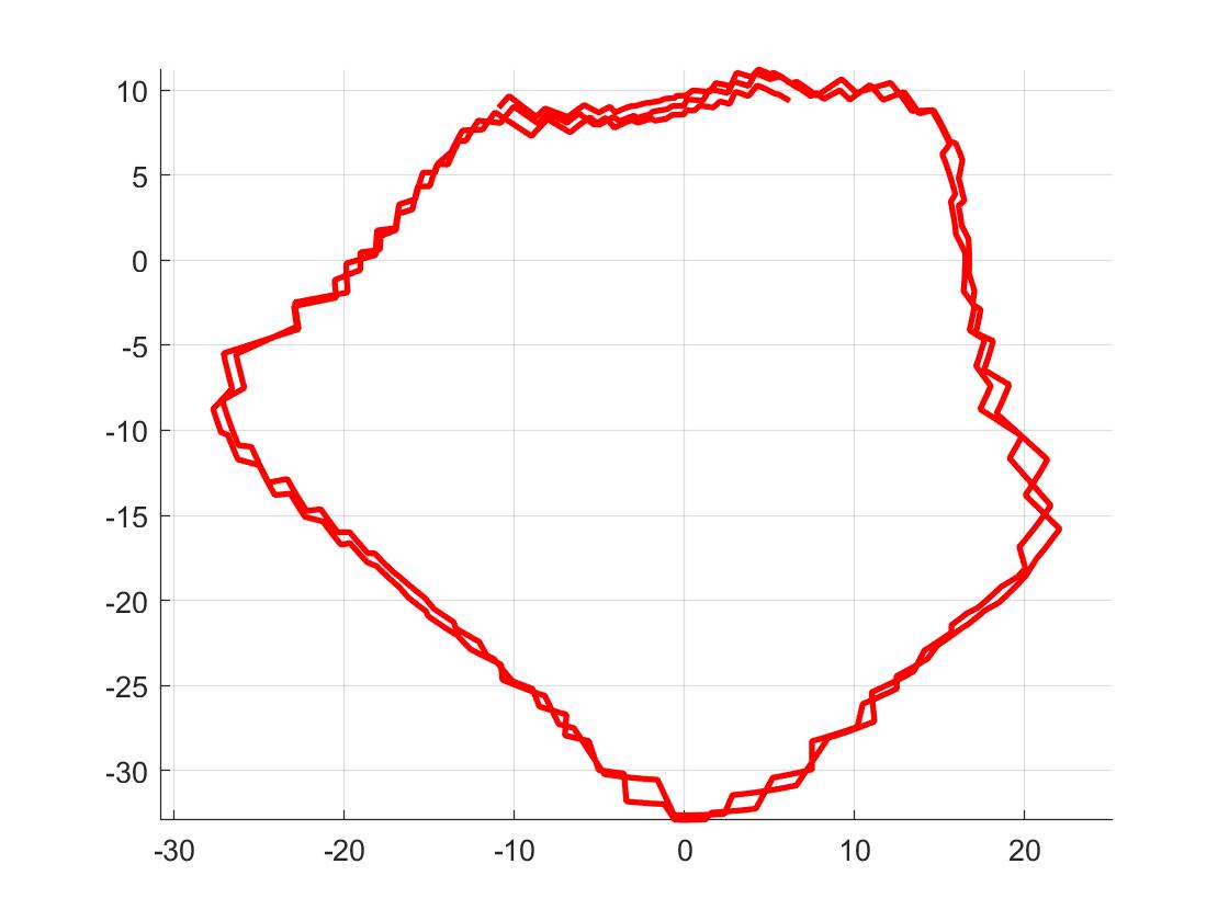
I converted the measurements from distance sensor to the inertial reference frame of the room:
Code (MATLAB):
% Lab 7 - 4960 clear; close all; clc % Part 1: Polar coordinates data = csvread('Lab7- Rotate_data (2).csv'); t = data(2:end,1); th = deg2rad(data(2:end,2)); dist = data(2:end,3); polarplot(th,dist,'linewidth',2) % Part 2 - Convert to inertial frame for i = 1:length(t) % Transformation matrix T = [cos(th(i)),-sin(th(i)),0; sin(th(i)),cos(th(i)),0; 0,0,1]; % Relative to ToF sensor rToF = [dist(i);0;1]; % Relative to inertial frame r_inertial =T*rToF; xi(i) = r_inertial(1); yi(i) = r_inertial(2); end figure; hold on; grid on; axis equal; plot(xi,yi,'r-','linewidth',2) hold off -
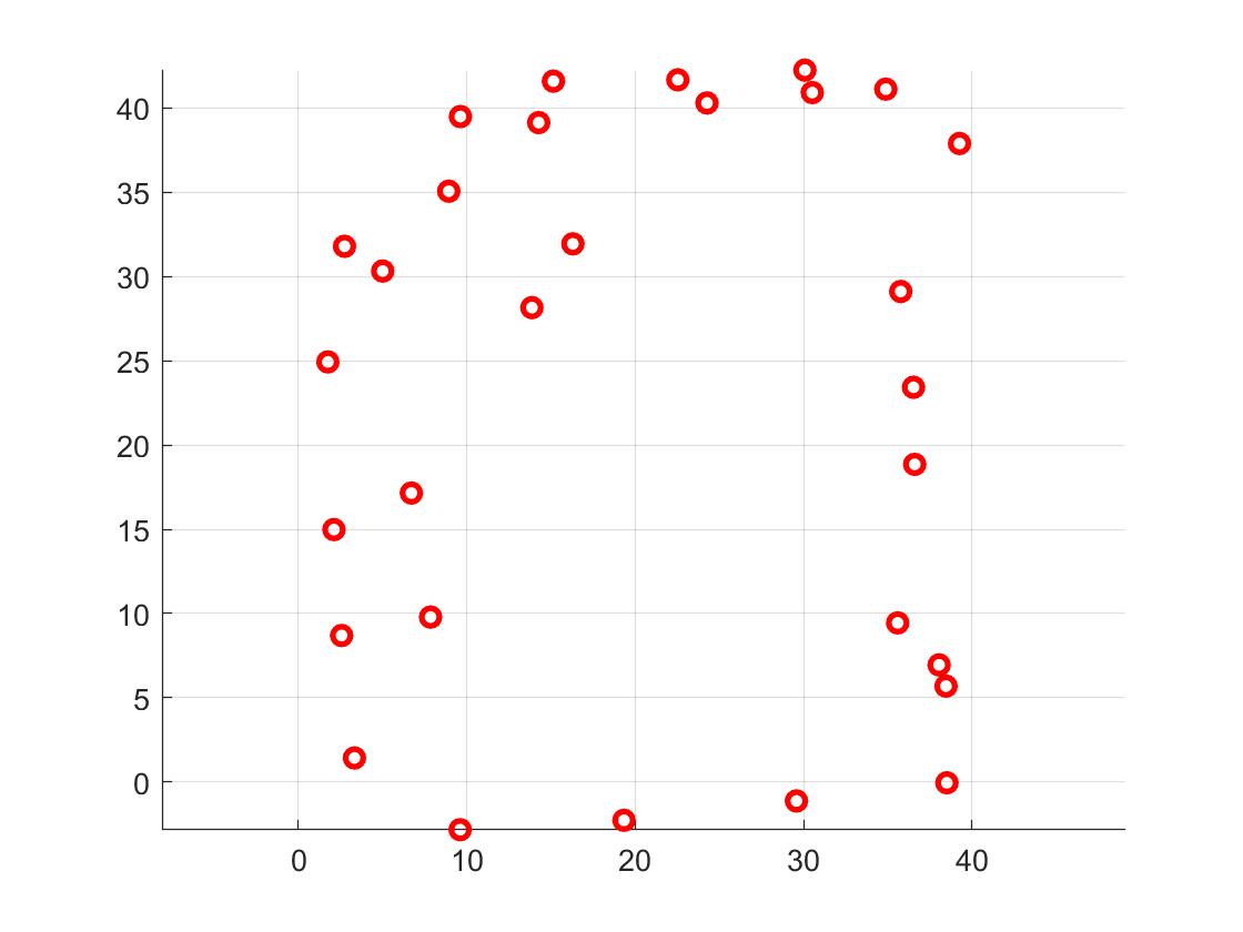
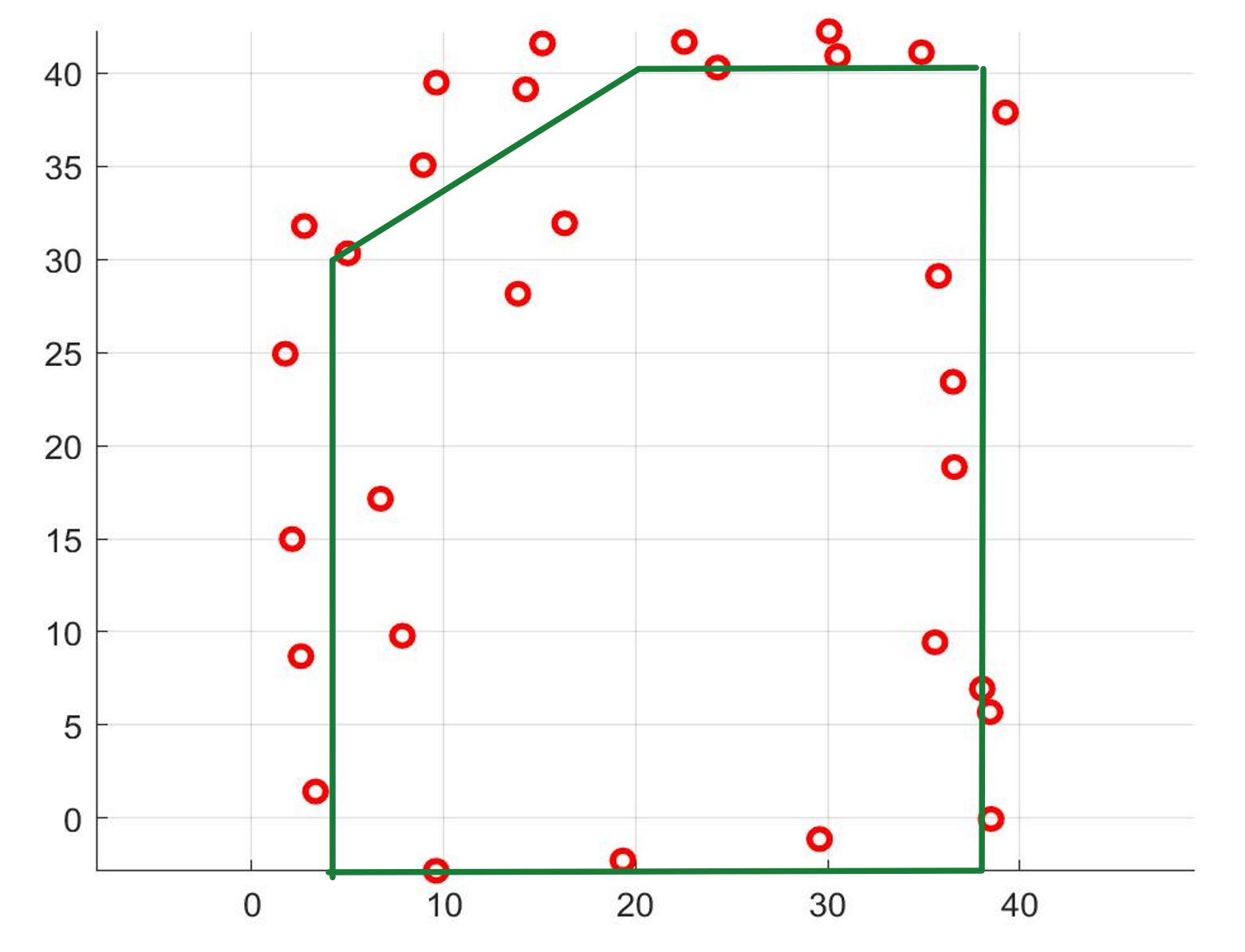
Finally, I built a map by manually placing the robot in known poses and plotting the scatter points using there measurements:
Finally, to convert this into a format I can use in the simulator, I manually guessed where the actual walls/obstacles are based on the scatter plot above.
I drew lines on top of these, and saved two lists of the end points of these lines:
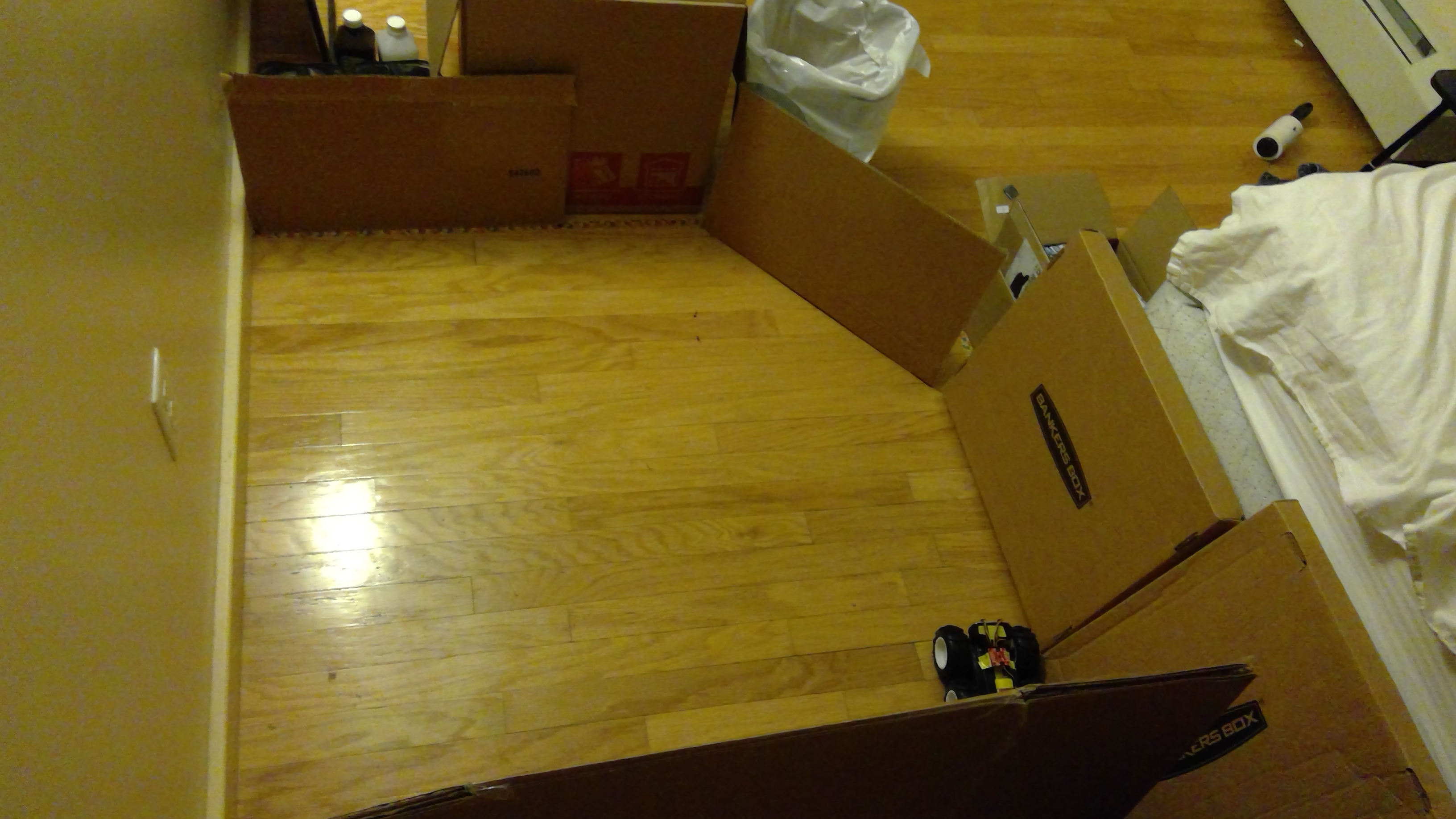
This is a very close representation of the actual map as shown here:
Map and points on the VM:
Code:
To account for the limited number (18) of readings allowed, I would interpolate the values between - 180 to + 180 degrees. This will ensure the spacing between the 18 readings to be accurate.# Start points for each line segment describing the map start_points = np.array([[4.5, 0], [4.5,30], [20, 40], [38,40], [38, 0]]) # End points for each line segment describing the map end_points = np.array([[4.5,30], [20, 40], [38,40], [38, 0], [4.5,0]]) # Check if map described by start_points and end_points is valid if(not is_map_valid(start_points, end_points)): raise Exception("The definitions of start_points and end_points are not valid. Please make sure the number of points are equal.")
